Jump to: Navigation
A case where prospective matching may limit bias in a randomized trial
A case where prospective matching may limit bias in a randomized trial
Cohort 연구의 경우 (전향적 연구)
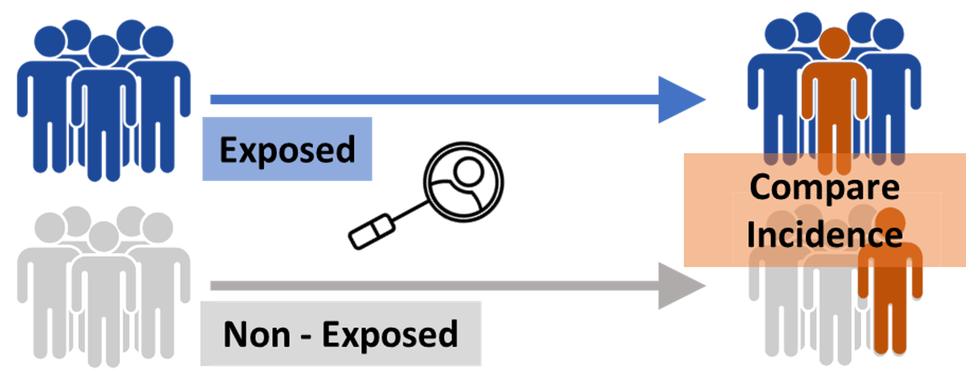
전향적 연구는 연구 시점에서 요인(치료, 위험인자)이 있는 사람과 없는 사람을 모아서, 결과 발생을 현 시점에서 시간의 경과와 더불어 추적해 가는 방법이다. 위험인자, 예후의 해석에 적합하다. Bias가 적은 것이 장점이지만 수고와 시간이 많이 걸린다.
Case Control 연구의 경우 (후향적 연구)
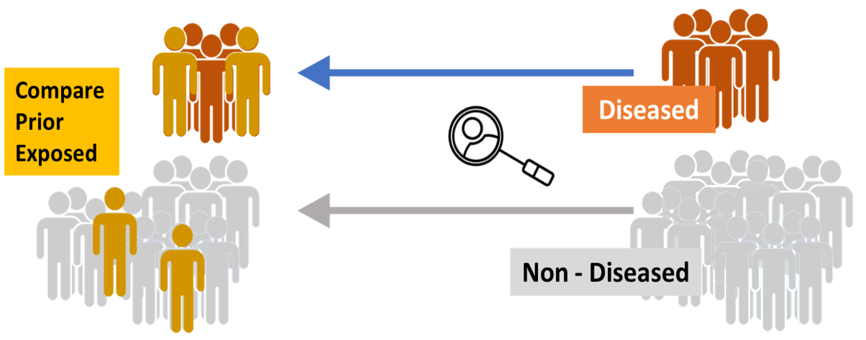
후향적 연구는 현재의 결과에서 시작되어 시간을 거슬러 올라가서 과거 요인의 유무를 해석하는 방법이다. 인과관계 발견에 적합하고, 노력이 적게 들지만, 연구자가 임의로 환자를 선택하게 되기 쉬워서 bias가 커지는 결점이 있다.
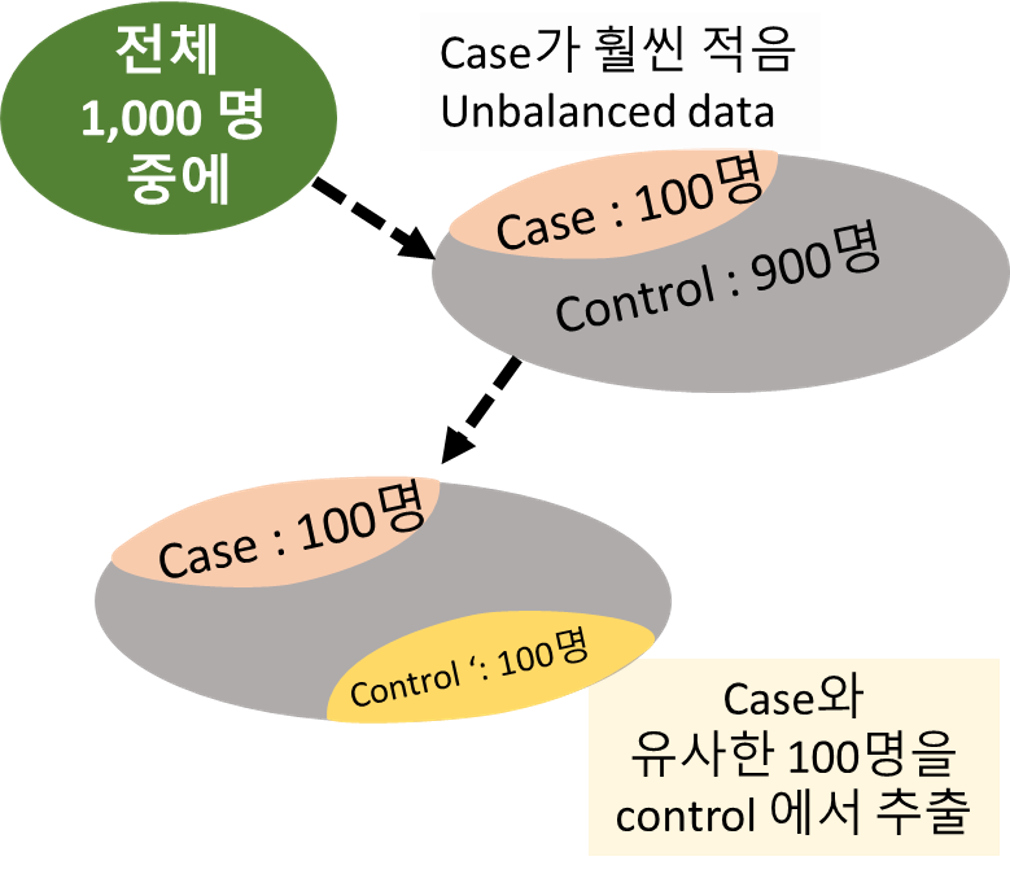
Case 군과 control 군의 base characteristics가 맞지 않음.
Case 군의 임상적 특징을 갖는 대상을 control 군 내에서 골라 Baseline 특성을 맞추어 주는 작업이 필요
If not, 선택 편향(selection bias) 발생
Matching의 필요성 예시
- 과연 control을 어떻게 설정할 것인가? *
Ex) 경구피임약이 유방암에 미치는 영향을 조사 시
- Case: 유방암이 발생한 여성

- Control : 유방암이 발생하지 않은 모든 여성
어린 초등학생들도 control 에 포함되어야 할까?
공변량(Covariate)들의 수준을 맞추어 통제한 후, 특정 독립변수가 종속변수에 미치는 영향의 정도를 제대로 파악할 수 있도록 하는 방법 : “ PSM “
(공변량은 여러 변인들이 공통적으로 공유하는 변량을 의미)
Article summary : The matching strategy
Analysis is important, but study design is paramount.
- 데이터에서 한 사람을 추출하여 나머지 사람들과 매칭시켜본다.
매칭 시에 고려되는 공변량 : 연구자의 생각에 기초하여 선정
such as age, gender, and one or two other relevant baseline measures.
2-1) 만약 매칭되는 사람이 없다면, 그 사람은 연구에서 제외.
2-2) 매칭되는 사람이 있다면, 첫 번째 개인은 therapy 그룹으로, 매칭된 사람은 control 그룹으로 배정
- 모든 사람이 matched되었거나, unmatched 그룹으로 할당될 때 까지 반
Library
library(dplyr)
library(data.table)
library(wakefield)
library(ggplot2)
library(knitr)
library(Matching)
- Matching Library
Multivariate and Propensity Score Matching with Balance Optimization
Data generation
300명의 simulated data를 생성 , ID와 성별(남자 70%, 여자 30%)과, 20세 부터 65세까지의 연령, BMI는 평균 25, 분산 3인 normal 분포 따르도록 생성
set.seed(1227)
dsamp <- r_data_frame(n = 300,
                      id,
                      sex(x = c(0,1),
                          prob = c(0.7,0.3),
                          name = "female"),
                      age(x = 20:65,
                          name = 'Age'),
                      Scoring=rnorm(300,25,3))

colnames(dsamp) <- c("ID","female","Age","BMI")
dsamp$BMI <-round(dsamp$BMI, 2)
dsamp$female  <- as.numeric(dsamp$female)-1
dsamp <- dsamp %>% as.data.table()
dsamp %>% head %>% kable()
| ID | female | Age | BMI |
|---|---|---|---|
| 001 | 0 | 52 | 25.63 |
| 002 | 1 | 50 | 26.81 |
| 003 | 1 | 32 | 24.09 |
| 004 | 1 | 59 | 21.79 |
| 005 | 0 | 49 | 24.88 |
| 006 | 0 | 62 | 25.93 |
The matching algorithm
dsamp[, rx := 0]
dused <- NULL
drand <- NULL
dcntl <- NULL
set.seed(1227)
while (nrow(dsamp) > 1) {

  selectRow <- sample(1:nrow(dsamp), 1)

  dsamp[selectRow, rx := 1]

  myTr <- dsamp[, rx]
  myX <- as.matrix(dsamp[, .(female, Age, BMI)])

  match.dt <- Match(Tr = myTr, X = myX,
                    caliper = c(0,0.5,0.5), ties = FALSE)
  # Ideally, we would want to have exact matches,
  # but this is unrealistic for continuous measures.
  # So, for age and BMI, we set the matching range to be 0.5 standard deviations.
  # (We do match exactly on gender.)

  if (length(match.dt) == 1) {  # no match

    dused <- rbind(dused, dsamp[selectRow])
    dsamp <- dsamp[-selectRow, ]

  } else {                      # match

    trt <- match.dt$index.treated
    ctl <- match.dt$index.control

    drand <- rbind(drand, dsamp[trt])
    dcntl <- rbind(dcntl, dsamp[ctl])

    dsamp <- dsamp[-c(trt, ctl)]

  }
}
Treatment 그룹에 할당된 데이터
drand %>% group_by(female) %>% summarize(mean_of_BMI = mean(BMI), count=n()) %>% kable
| female | mean_of_BMI | count |
|---|---|---|
| 0 | 25.21000 | 102 |
| 1 | 24.96757 | 37 |
Control 그룹에 할당된 데이터
dcntl %>% group_by(female) %>% summarize(mean_of_BMI = mean(BMI), count=n())%>% kable()
| female | mean_of_BMI | count |
|---|---|---|
| 0 | 25.23196 | 102 |
| 1 | 24.88054 | 37 |
만들어진 데이터 형태
drand %>% head()%>% kable()
| ID | female | Age | BMI | rx |
|---|---|---|---|---|
| 119 | 0 | 32 | 23.91 | 1 |
| 212 | 1 | 39 | 20.36 | 1 |
| 245 | 0 | 21 | 28.34 | 1 |
| 036 | 1 | 23 | 23.35 | 1 |
| 086 | 1 | 37 | 21.66 | 1 |
| 113 | 0 | 35 | 22.65 | 1 |
dcntl %>% head()%>% kable()
| ID | female | Age | BMI | rx |
|---|---|---|---|---|
| 100 | 0 | 32 | 23.93 | 0 |
| 256 | 1 | 36 | 20.05 | 0 |
| 257 | 0 | 24 | 28.42 | 0 |
| 186 | 1 | 20 | 23.29 | 0 |
| 211 | 1 | 35 | 22.00 | 0 |
| 260 | 0 | 35 | 22.96 | 0 |
treatment 그룹과 control 그룹의 짝을 연결
mtanum이라는 변수를 이용
dused는 매칭되지 않은 데이터
drand$matnum <- c(1:dim(drand)[1])
dcntl$matnum <- c(1:dim(dcntl)[1])

dused1 <- dused
dused1$matnum <-NA
tt <- bind_rows(as.data.frame(drand),as.data.frame(dcntl))
tt %>% arrange(matnum) %>% head %>% kable()
| ID | female | Age | BMI | rx | matnum |
|---|---|---|---|---|---|
| 119 | 0 | 32 | 23.91 | 1 | 1 |
| 100 | 0 | 32 | 23.93 | 0 | 1 |
| 212 | 1 | 39 | 20.36 | 1 | 2 |
| 256 | 1 | 36 | 20.05 | 0 | 2 |
| 245 | 0 | 21 | 28.34 | 1 | 3 |
| 257 | 0 | 24 | 28.42 | 0 | 3 |
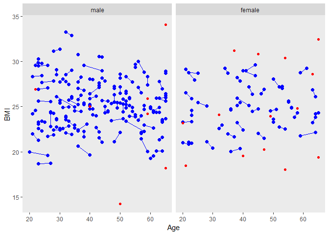
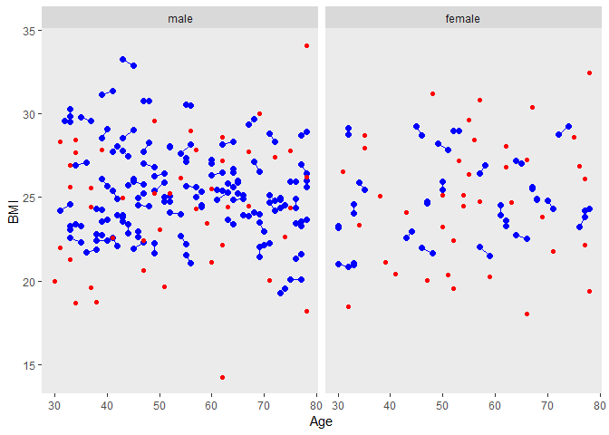
labels <- c("0" = "male", "1" = "female")

ggplot(tt,aes(Age, BMI, group=matnum))+
  geom_point(size=2, colour="blue")+
  geom_line(colour="blue")+ facet_grid( ~ female, labeller=labeller(female = labels))+
  theme(panel.grid.major = element_blank(), panel.grid.minor = element_blank())+
  geom_point(data=dused1, aes(Age, BMI, group=matnum),color="red")
male의 trt vs control group 비교
tt %>% filter(female==0) %>%
  group_by(rx) %>%
  summarize(count=n(),mu.age=mean(Age),sd.age=sd(Age),mu.BMI=mean(BMI),sd.BMI=sd(Age))%>%
  kable()
| rx | count | mu.age | sd.age | mu.BMI | sd.BMI |
|---|---|---|---|---|---|
| 0 | 102 | 42.56863 | 13.08049 | 25.23196 | 13.08049 |
| 1 | 102 | 42.51961 | 13.51620 | 25.21000 | 13.51620 |
female의 trt vs control group 비교
tt %>% filter(female==1) %>%
  group_by(rx) %>%
  summarize(count=n(),mu.age=mean(Age),sd.age=sd(Age),mu.BMI=mean(BMI),sd.BMI=sd(Age))%>%
  kable()
| rx | count | mu.age | sd.age | mu.BMI | sd.BMI |
|---|---|---|---|---|---|
| 0 | 37 | 41.94595 | 13.85028 | 24.88054 | 13.85028 |
| 1 | 37 | 41.62162 | 13.39227 | 24.96757 | 13.39227 |
The distributions of the matching variables (or least the means and standard deviations) appear quite close, as we can see by looking at the males and females separately.
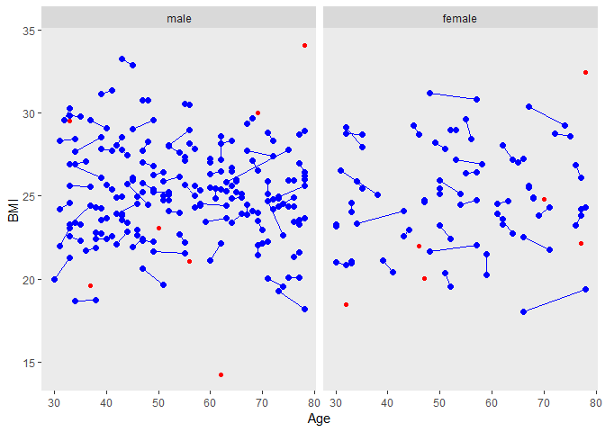
caliper values 에 따른 비교
1. caliper = c(0,0.5,0.5) ⇒ c(0,0.2,0.2)
We could get shorter line segments if we reduced the caliper values, but we would certainly increase the number of unmatched patients.
set.seed(1227)
dsamp <- r_data_frame(n = 300,
                      id,
                      sex(x = c(0,1),
                          prob = c(0.7,0.3),
                          name = "female"),
                      age(x = 30:78,
                          name = 'Age'),
                      Scoring=rnorm(300,25,3))

colnames(dsamp) <- c("ID","female","Age","BMI")
dsamp$BMI <-round(dsamp$BMI, 2)
dsamp$female  <- as.numeric(dsamp$female)-1
dsamp <- dsamp %>% as.data.table()

dsamp[, rx := 0]
dused <- NULL
drand <- NULL
dcntl <- NULL


set.seed(1227)
while (nrow(dsamp) > 1) {
  selectRow <- sample(1:nrow(dsamp), 1)
  dsamp[selectRow, rx := 1]
  myTr <- dsamp[, rx]
  myX <- as.matrix(dsamp[, .(female, Age, BMI)])

  match.dt <- Match(Tr = myTr, X = myX,
                    caliper = c(0,0.2,0.2), ties = FALSE)

  if (length(match.dt) == 1) {  # no match
    dused <- rbind(dused, dsamp[selectRow])
    dsamp <- dsamp[-selectRow, ]
  } else {                      # match
    trt <- match.dt$index.treated
    ctl <- match.dt$index.control
    drand <- rbind(drand, dsamp[trt])
    dcntl <- rbind(dcntl, dsamp[ctl])
    dsamp <- dsamp[-c(trt, ctl)]
  }
}

drand$matnum <- c(1:dim(drand)[1])
dcntl$matnum <- c(1:dim(dcntl)[1])

dused1 <- dused
dused1$matnum <-NA
tt <- bind_rows(as.data.frame(drand),as.data.frame(dcntl))
labels <- c("0" = "male", "1" = "female")

ggplot(tt,aes(Age, BMI, group=matnum))+
  geom_point(size=2, colour="blue")+
  geom_line(colour="blue")+ facet_grid( ~ female, labeller=labeller(female = labels))+
  theme(panel.grid.major = element_blank(), panel.grid.minor = element_blank())+
  geom_point(data=dused1,aes(Age, BMI, group=matnum),color="red")
2. caliper = c(0,0.5,0.5) ⇒ c(0,0.9,0.9)
DALEX has a new skin!
DALEX has a new skin!
DALEX (Descriptive mAchine Learning EXplanations)

DALEX is an R package for visual explanation, exploration, diagnostic and debugging of predictive ML models

Recently Hanna Dyrcz designed a new beautiful theme for these explainers. Hanna is a very talented designer.
devtools::install_github("pbiecek/DALEX")
library(knitr); library(dplyr)
library(randomForest)
library(e1071)
library(rms)
library(gbm)
library(caret); library(data.table)
library("DALEX")
titanic <- na.omit(titanic)
titanic %>% head %>%  kable()
| gender | age | class | embarked | country | fare | sibsp | parch | survived |
|---|---|---|---|---|---|---|---|---|
| male | 42 | 3rd | Southampton | United States | 7.11 | 0 | 0 | no |
| male | 13 | 3rd | Southampton | United States | 20.05 | 0 | 2 | no |
| male | 16 | 3rd | Southampton | United States | 20.05 | 1 | 1 | no |
| female | 39 | 3rd | Southampton | England | 20.05 | 1 | 1 | yes |
| female | 16 | 3rd | Southampton | Norway | 7.13 | 0 | 0 | yes |
| male | 25 | 3rd | Southampton | United States | 7.13 | 0 | 0 | yes |
모델 준비
model_titanic_rf <- randomForest(as.factor(survived == "yes") ~ gender + age + class + embarked +
                                 fare + sibsp + parch,  data = titanic)

explain_titanic_rf <- explain(model_titanic_rf,
                              data = titanic[,-9],
                              y = titanic$survived == "yes",
                              label = "Random Forest v7")

vi_rf <- variable_importance(explain_titanic_rf)
plot(vi_rf)

기존의 variable importance plot과의 비교
library(caret)
varImpPlot(model_titanic_rf,type=2)
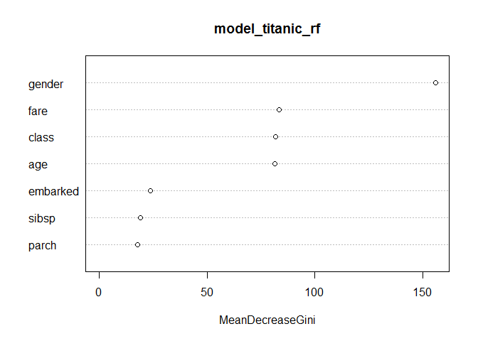
변수의 효과
Gender가 가장 중요한 변수
class, Age , Fare 가 그 다음 중요한 세가지 변수
모델의 반응과 이 변수들 사이의 관계를 보고자 한다.
“univariate relation” : can be calculated with variable_response()
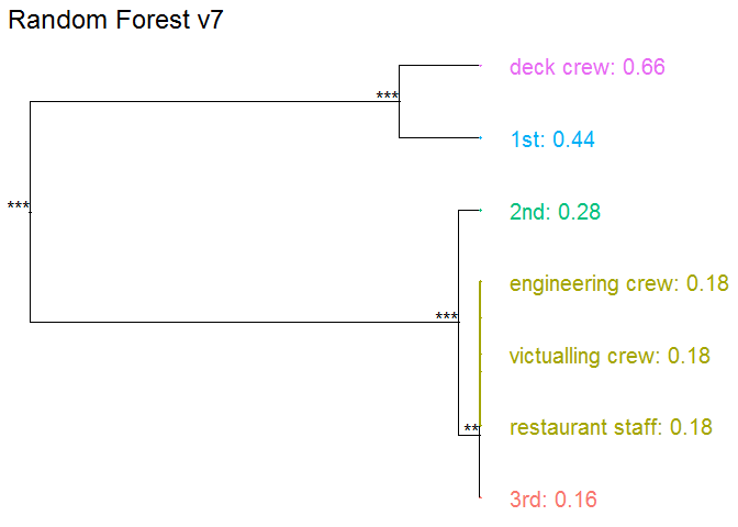
Passanger class
Passangers in the first class have much higher survival probability.
vr_class  <- variable_response(explain_titanic_rf, variable =  "class", type="factor")
plot(vr_class)
## Scale for 'x' is already present. Adding another scale for 'x', which
## will replace the existing scale.
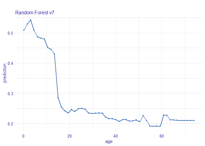
Age
5살 이하의 어린이들이 살 확률이 더 높았다.
vr_age  <- variable_response(explain_titanic_rf, variable =  "age")
plot(vr_age, use_facets = TRUE)
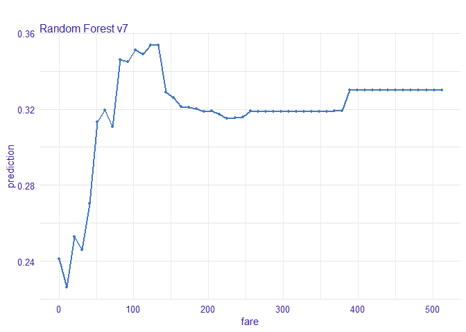
Fare
가장 저렴한 티켓은 낮은 생존 확률과 연관되어 있다.
vr_fare  <- variable_response(explain_titanic_rf, variable =  "fare")
plot(vr_fare, use_facets = TRUE)
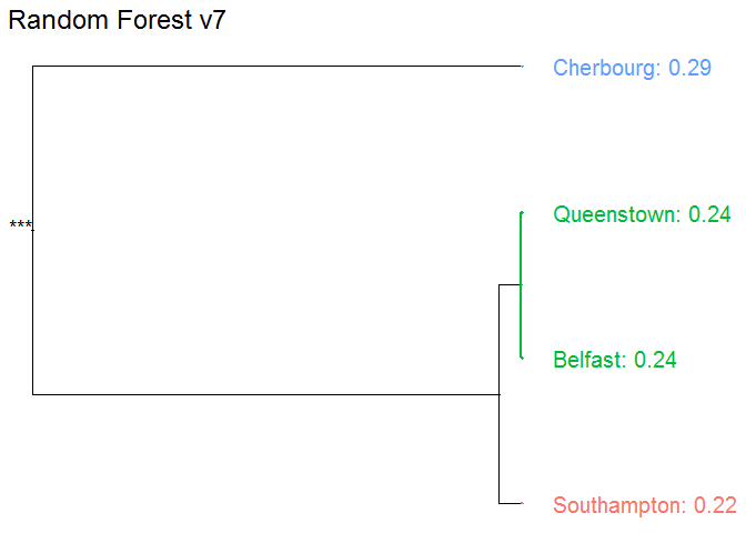
Embarked
Cherbourg에서의 탑승객들이 가장 높은 생존을 보인다.
vr_embarked  <- variable_response(explain_titanic_rf, variable =  "embarked", type="factor")
plot(vr_embarked)
## Scale for 'x' is already present. Adding another scale for 'x', which
## will replace the existing scale.
Instance level explanations
Let’s see break down explanation for model predictions for 8 years old male from 1st class that embarked from port C.
new_passanger <- data.frame(
  class = factor("1st", levels = c("1st", "2nd", "3rd", "deck crew", "engineering crew", "restaurant staff", "victualling crew")),
  gender = factor("male", levels = c("female", "male")),
  age = 8,
  sibsp = 0,
  parch = 0,
  fare = 72,
  embarked = factor("Southampton", levels = c("Belfast", "Cherbourg", "Queenstown", "Southampton"))
)

new_passanger %>% kable()
| class | gender | age | sibsp | parch | fare | embarked |
|---|---|---|---|---|---|---|
| 1st | male | 8 | 0 | 0 | 72 | Southampton |
sp_rf <- single_prediction(explain_titanic_rf, new_passanger)
plot(sp_rf)
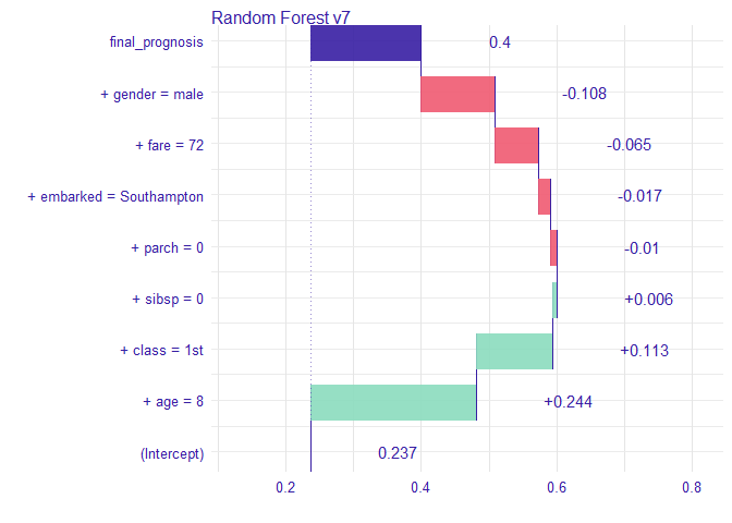
이 탑승객에게 가장 중요한 변수는 나이와 성별로 보인다. 전반적으로 이 탑승객의 생존 odds는 평균적인 탑승객보다 높음을 알 수 있다. 주된 요인은 남자임에도 어린 나이 때문인 것으로 생각된다.
다양한 모델들
Logistic regression
model_titanic_lmr <- lrm(survived == "yes" ~ class + gender + rcs(age) + sibsp +
                           parch + fare + embarked, titanic)
explain_titanic_lmr <- explain(model_titanic_lmr, data = titanic,
                               y = titanic$survived == "yes",
                               predict_function = function(m,x) predict(m, x, type="fitted"),
                               label = "Logistic regression")
Generalized Boosted Models (GBM)
model_titanic_gbm <- gbm(survived == "yes" ~ class + gender + age + sibsp +
                           parch + fare + embarked, data = titanic, n.trees = 15000)
## Distribution not specified, assuming bernoulli ...
explain_titanic_gbm <- explain(model_titanic_gbm, data = titanic,
                               y = titanic$survived == "yes",
                               predict_function = function(m,x) predict(m, x, n.trees = 15000, type = "response"),
                               label = "Generalized Boosted Models")
Support Vector Machines (SVM)
model_titanic_svm <- svm(survived == "yes" ~ class + gender + age + sibsp +
                           parch + fare + embarked, data = titanic,
                         type = "C-classification", probability = TRUE)
explain_titanic_svm <- explain(model_titanic_svm, data = titanic,
                               y = titanic$survived == "yes",
                               label = "Support Vector Machines")
k-Nearest Neighbours (kNN)
model_titanic_knn <- knn3(survived == "yes" ~ class + gender + age + sibsp +
                            parch + fare + embarked, data = titanic, k = 5)
explain_titanic_knn <- explain(model_titanic_knn, data = titanic,
                               y = titanic$survived == "yes",
                               predict_function = function(m,x) predict(m, x)[,2],
                               label = "k-Nearest Neighbours")
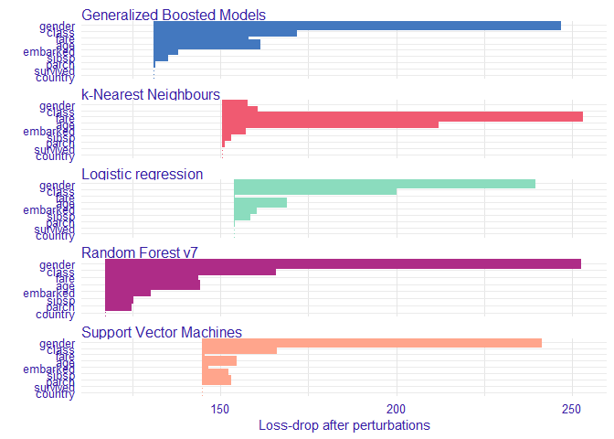
Variable performance
vi_rf <- variable_importance(explain_titanic_rf)
vi_lmr <- variable_importance(explain_titanic_lmr)
vi_gbm <- variable_importance(explain_titanic_gbm)
vi_svm <- variable_importance(explain_titanic_svm)
vi_knn <- variable_importance(explain_titanic_knn)

plot(vi_rf, vi_lmr, vi_gbm, vi_svm, vi_knn, bar_width = 4)
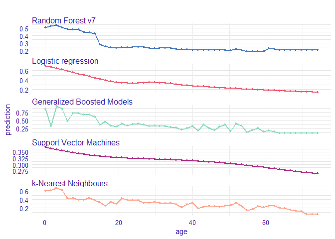
Single variable
vr_age_rf  <- variable_response(explain_titanic_rf, variable =  "age")
vr_age_lmr  <- variable_response(explain_titanic_lmr, variable =  "age")
vr_age_gbm  <- variable_response(explain_titanic_gbm, variable =  "age")
vr_age_svm  <- variable_response(explain_titanic_svm, variable =  "age")
vr_age_knn  <- variable_response(explain_titanic_knn, variable =  "age")
plot(vr_age_rf, vr_age_lmr, vr_age_gbm, vr_age_svm, vr_age_knn)
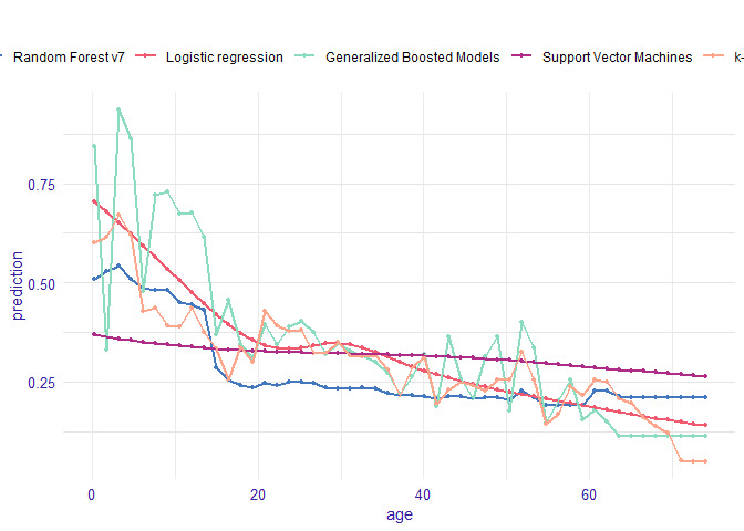
plot(vr_age_rf, vr_age_lmr, vr_age_gbm, vr_age_svm, vr_age_knn, use_facets = TRUE)
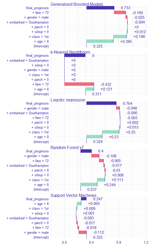
Instance level explanations
sp_rf <- single_prediction(explain_titanic_rf, new_passanger)
sp_lmr <- single_prediction(explain_titanic_lmr, new_passanger)
sp_gbm <- single_prediction(explain_titanic_gbm, new_passanger)
sp_svm <- single_prediction(explain_titanic_svm, new_passanger)
sp_knn <- single_prediction(explain_titanic_knn, new_passanger)
plot(sp_rf, sp_lmr, sp_gbm, sp_svm, sp_knn)
Hello
Cum sociis natoque penatibus et magnis dis parturient montes, nascetur ridiculus mus. Aenean eu leo quam. Pellentesque ornare sem lacinia quam venenatis vestibulum. Sed posuere consectetur est at lobortis. Cras mattis consectetur purus sit amet fermentum.
Sunny first posts
Hi
Features
Features include:
- Touch-enabled sidebar / drawer for mobile, including fallback when JS is disabled.
- Github Pages compatible tag support based on this post.
- Customizable link color and sidebar image, per-site, per-tag and per-post.
- Optional author section at the bottom of each post.
- Optional comment section powered by Disqus.
- Layout for posts grouped by year
- Wide array of social media icons on sidebar.
- Math blocks via KaTeX.